텐서플로 튜토리얼(1)-기본 이미지 분류

텐서플로 튜토리얼(1)-기본 이미지 분류

참고링크

머신러닝	딥러닝	선형대수	기초통계	최적화
k-means	신경망이란	고유값,고유벡터	확률변수	컨벡스 셋
k-최근접이웃	성능함수	행렬식	확률분포	컨벡스 함수
선형회귀	신경망 학습	내적	모집단과 표본	라그랑주 듀얼
로지스틱회귀	교차연결	기저	평균과 분산	KKT 조건
릿지,라쏘회귀	합성곱 신경망	랭크, 차원	공분산, 상관계수	ROC 커브
의사결정나무	배치, 에포크 차이	선형변환	최대가능도추정	크로스 밸리데이션
서포트벡터머신	텐서플로기초(1)	직교행렬	베르누이,이항분포	실루엣 스코어
원클래스 SVM	텐서플로기초(2)	고유값분해	기하,음이항분포
LDA	seq2seq	특이값분해	초기하분포
GMM	opencv기초		포아송분포
부스팅	resnet		정규분포
사이킷런 실습	다각형내부판별		감마분포
	엣지판별		지수분포
			카이제곱분포
			베타분포
			균일분포

본 포스팅은 텐서플로 튜토리얼과 동일한 내용입니다.

import 라이브러리

from __future__ import absolute_import, division, print_function, unicode_literals, unicode_literals

# tensorflow와 tf.keras를 임포트합니다
import tensorflow as tf
from tensorflow import keras

import numpy as np
import matplotlib.pyplot as plt

print(tf.__version__)

2.0.0

전체 데이터 모양

train, test 분리

fashion_mnist = keras.datasets.fashion_mnist

(train_images, train_labels), (test_images, test_labels) = fashion_mnist.load_data()

Downloading data from https://storage.googleapis.com/tensorflow/tf-keras-datasets/train-labels-idx1-ubyte.gz
32768/29515 [=================================] - 0s 3us/step
Downloading data from https://storage.googleapis.com/tensorflow/tf-keras-datasets/train-images-idx3-ubyte.gz
26427392/26421880 [==============================] - 10s 0us/step
Downloading data from https://storage.googleapis.com/tensorflow/tf-keras-datasets/t10k-labels-idx1-ubyte.gz
8192/5148 [===============================================] - 0s 0us/step
Downloading data from https://storage.googleapis.com/tensorflow/tf-keras-datasets/t10k-images-idx3-ubyte.gz
4423680/4422102 [==============================] - 1s 0us/step

데이터 확인

class_names = ['T-shirt/top', 'Trouser', 'Pullover', 'Dress', 'Coat',
               'Sandal', 'Shirt', 'Sneaker', 'Bag', 'Ankle boot']

아래 결과는 train 데이터는 28x28 이미지가 60,000장 이라는 뜻입니다.

train_images.shape

(60000, 28, 28)

len(train_labels)

60000

train_labels

array([9, 0, 0, ..., 3, 0, 5], dtype=uint8)

test_images.shape

(10000, 28, 28)

len(test_labels)

10000

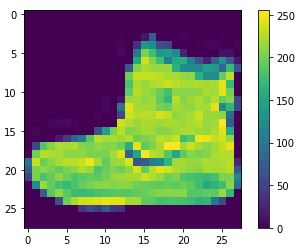
plt.figure()
plt.imshow(train_images[0])
plt.colorbar()
plt.grid(False)
plt.show()

train_images = train_images / 255.0
test_images = test_images / 255.0

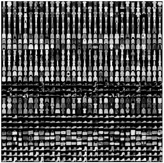
plt.figure(figsize=(10,10))
for i in range(25):
    plt.subplot(5,5,i+1)
    plt.xticks([])
    plt.yticks([])
    plt.grid(False)
    plt.imshow(train_images[i], cmap=plt.cm.binary)
    plt.xlabel(class_names[train_labels[i]])
plt.show()

model = keras.Sequential([
    keras.layers.Flatten(input_shape=(28, 28)),
    keras.layers.Dense(128, activation='relu'),
    keras.layers.Dense(10, activation='softmax')
])

model.compile(optimizer='adam',
              loss='sparse_categorical_crossentropy',
              metrics=['accuracy'])

model.fit(train_images, train_labels, epochs=5)

Train on 60000 samples
Epoch 1/5
60000/60000 [==============================] - 6s 99us/sample - loss: 0.4996 - accuracy: 0.8248
Epoch 2/5
60000/60000 [==============================] - 5s 82us/sample - loss: 0.3755 - accuracy: 0.8634
Epoch 3/5
60000/60000 [==============================] - 5s 80us/sample - loss: 0.3367 - accuracy: 0.8780
Epoch 4/5
60000/60000 [==============================] - 5s 75us/sample - loss: 0.3125 - accuracy: 0.8856
Epoch 5/5
60000/60000 [==============================] - 5s 82us/sample - loss: 0.2943 - accuracy: 0.8913

test_loss, test_acc = model.evaluate(test_images,  test_labels, verbose=2)

print('\n테스트 정확도:', test_acc)

10000/1 - 1s - loss: 0.2947 - accuracy: 0.8728

테스트 정확도: 0.8728

predictions = model.predict(test_images)

predictions[0]

array([1.6788504e-06, 5.5685239e-09, 8.1212349e-08, 1.3833268e-08,
       1.4137331e-07, 2.8559810e-02, 9.8572048e-07, 2.8257709e-02,
       3.2442263e-06, 9.4317627e-01], dtype=float32)

np.argmax(predictions[0])

9

test_labels[0]

9

def plot_image(i, predictions_array, true_label, img):
    predictions_array, true_label, img = predictions_array[i], true_label[i], img[i]
    plt.grid(False)
    plt.xticks([])
    plt.yticks([])

    plt.imshow(img, cmap=plt.cm.binary)

    predicted_label = np.argmax(predictions_array)
    if predicted_label == true_label:
        color = 'blue'
    else:
        color = 'red'

    plt.xlabel("{} {:2.0f}% ({})".format(class_names[predicted_label],
                                100*np.max(predictions_array),
                                class_names[true_label]),
                                color=color)

def plot_value_array(i, predictions_array, true_label):
    predictions_array, true_label = predictions_array[i], true_label[i]
    plt.grid(False)
    plt.xticks([])
    plt.yticks([])
    thisplot = plt.bar(range(10), predictions_array, color="#777777")
    plt.ylim([0, 1])
    predicted_label = np.argmax(predictions_array)

    thisplot[predicted_label].set_color('red')
    thisplot[true_label].set_color('blue')

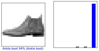
i = 0
plt.figure(figsize=(6,3))
plt.subplot(1,2,1)
plot_image(i, predictions, test_labels, test_images)
plt.subplot(1,2,2)
plot_value_array(i, predictions,  test_labels)
plt.show()

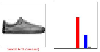
i = 12
plt.figure(figsize=(6,3))
plt.subplot(1,2,1)
plot_image(i, predictions, test_labels, test_images)
plt.subplot(1,2,2)
plot_value_array(i, predictions,  test_labels)
plt.show()

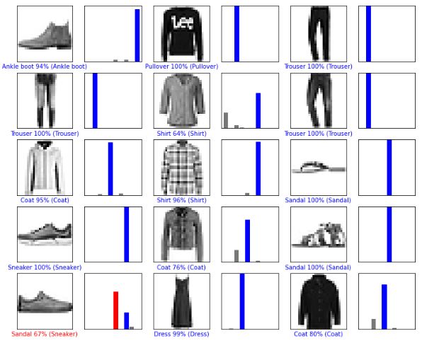
# 처음 X 개의 테스트 이미지와 예측 레이블, 진짜 레이블을 출력합니다
# 올바른 예측은 파랑색으로 잘못된 예측은 빨강색으로 나타냅니다
num_rows = 5
num_cols = 3
num_images = num_rows*num_cols
plt.figure(figsize=(2*2*num_cols, 2*num_rows))
for i in range(num_images):
    plt.subplot(num_rows, 2*num_cols, 2*i+1)
    plot_image(i, predictions, test_labels, test_images)
    plt.subplot(num_rows, 2*num_cols, 2*i+2)
    plot_value_array(i, predictions, test_labels)
plt.show()

# 테스트 세트에서 이미지 하나를 선택합니다
img = test_images[0]

print(img.shape)

(28, 28)

# 이미지 하나만 사용할 때도 배치에 추가합니다
img = (np.expand_dims(img,0))

print(img.shape)

(1, 28, 28)

predictions_single = model.predict(img)

print(predictions_single)

[[1.6788470e-06 5.5685234e-09 8.1212491e-08 1.3833266e-08 1.4137342e-07
  2.8559841e-02 9.8571843e-07 2.8257780e-02 3.2442322e-06 9.4317615e-01]]

plot_value_array(0, predictions_single, test_labels)
_ = plt.xticks(range(10), class_names, rotation=45)

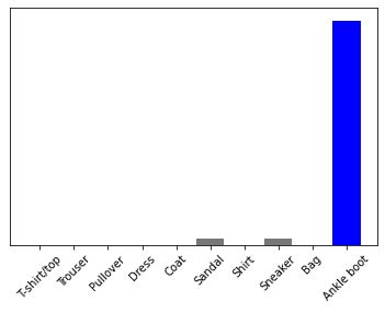
np.argmax(predictions_single[0])

9